Emissions trading is a market-based approach used to control
pollution by providing
economic incentives for achieving reductions in the emissions of
pollutants.
[1] It is a form of
carbon pricing.
A central authority (usually a
governmental body) sets a limit or
cap on the amount of a pollutant that can be emitted. The limit or cap is allocated or sold to firms in the form of emissions permits which represent the right to emit or discharge a specific volume of the specified pollutant. Firms are required to hold a number of permits (or
carbon credits) equivalent to their emissions. The total number of permits cannot exceed the cap, limiting total emissions to that level. Firms that need to increase their emission permits must buy permits from those who require fewer permits.
[1] The transfer of permits is referred to as a
trade. In effect, the buyer is paying a charge for polluting, while the seller is being rewarded for having reduced emissions. Thus, in theory, those who can reduce emissions most cheaply will do so, achieving the pollution reduction at the lowest cost to society.
[2]
By definition, an
externality is an activity of one entity that affects the welfare of another entity in a way that is outside the market mechanism.
[5] Pollution is the prime example most economists think of when discussing externalities. There are many different ways to address these from a public economics perspective including emissions fees, cap-and-trade, and command-and-control regulation. Here we will discuss cap-and-trade as the chosen public response to externalities.
[edit] Overview
The overall goal of an emissions trading plan is to minimize the cost of meeting a set emissions target.
[6] The
cap is an enforceable limit on emissions that is usually lowered over time — aiming towards a national emissions reduction target.
[6] In other systems a portion of all traded credits must be retired, causing a net reduction in emissions each time a trade occurs. In many cap-and-trade systems, organizations which do not pollute may also participate, thus
environmental groups can purchase and retire allowances or credits and hence drive up the price of the remainder according to the
law of demand.
[7] Corporations can also prematurely retire allowances by donating them to a nonprofit entity and then be eligible for a tax deduction.
[edit] Definitions
The economics literature provides the following definitions of cap and trade emissions trading schemes.
A cap-and-trade system constrains the aggregate emissions of regulated sources by creating a limited number of tradable emission allowances, which emission sources must secure and surrender in number equal to their emissions.[8]
In an emissions trading or cap-and-trade scheme, a limit on access to a resource (the cap) is defined and then allocated among users in the form of permits. Compliance is established by comparing actual emissions with permits surrendered including any permits traded within the cap.[9]
Under a tradable permit system, an allowable overall level of pollution is established and allocated among firms in the form of permits. Firms that keep their emission levels below their allotted level may sell their surplus permits to other firms or use them to offset excess emissions in other parts of their facilities.[10]
[edit] Market-based and least-cost
Economists have urged the use of "market-based" instruments such as emissions trading to address environmental problems instead of prescriptive "command and control" regulation.
[11] Command and control regulation is criticized for being excessively rigid, insensitive to geographical and technological differences, and for being inefficient.
[12] However, emissions trading requires a cap to effectively reduce emissions, and the cap is a government regulatory mechanism. After a cap has been set by a government political process, individual companies are free to choose how or if they will reduce their emissions. Failure to reduce emissions is often punishable by a further government regulatory mechanism, a fine that increases costs of production. Firms will choose the least-costly way to comply with the pollution regulation, which will lead to reductions where the least expensive solutions exist, while allowing emissions that are more expensive to reduce.
[edit] Emission markets
For trading purposes, one allowance or CER is considered equivalent to one
metric ton of CO
2 emissions. These allowances can be sold privately or in the international market at the prevailing market price. These trade and
settle internationally and hence allow allowances to be transferred between countries. Each international transfer is validated by the
UNFCCC. Each transfer of ownership within the European Union is additionally validated by the European Commission.
Climate exchanges have been established to provide a
spot market in allowances, as well as
futures and
options market to help discover a market price and maintain
liquidity. Carbon prices are normally quoted in
Euros per tonne of carbon dioxide or its equivalent (CO
2e). Other greenhouse gasses can also be traded, but are quoted as standard multiples of carbon dioxide with respect to their
global warming potential. These features reduce the quota's financial impact on business, while ensuring that the quotas are met at a national and international level.
Currently there are six exchanges trading in carbon allowances: the
Chicago Climate Exchange,
European Climate Exchange,
NASDAQ OMX Commodities Europe,
PowerNext,
Commodity Exchange Bratislava and the
European Energy Exchange. NASDAQ OMX Commodities Europe listed a contract to trade offsets generated by a CDM
carbon project called Certified Emission Reductions (CERs). Many companies now engage in emissions abatement, offsetting, and sequestration programs to generate credits that can be sold on one of the exchanges. At least one
private electronic market has been established in 2008: CantorCO2e.
[13] Carbon credits at Commodity Exchange Bratislava are traded at special platform - Carbon place.
[14]
Managing emissions is one of the fastest-growing segments in financial services in the
City of London with a market estimated to be worth about €30 billion in 2007. Louis Redshaw, head of environmental markets at
Barclays Capital predicts that "Carbon will be the world's biggest commodity market, and it could become the world's biggest market overall."
[15]
[edit] History
The efficiency of what later was to be called the "cap-and-trade" approach to
air pollution abatement was first demonstrated in a series of micro-economic computer simulation studies between 1967 and 1970 for the National Air Pollution Control Administration (predecessor to the
United States Environmental Protection Agency's Office of Air and Radiation) by Ellison Burton and William Sanjour. These studies used mathematical models of several cities and their emission sources in order to compare the cost and effectiveness of various control strategies.
[16][17][18][19][20] Each abatement strategy was compared with the "least cost solution" produced by a computer optimization program to identify the least costly combination of source reductions in order to achieve a given abatement goal.
[21] In each case it was found that the least cost solution was dramatically less costly than the same amount of pollution reduction produced by any conventional abatement strategy.
[22] Burton and later Sanjour along with Edward H. Pechan continued improving
[23]and advancing
[24] these computer models at the newly-created U.S. Environmental Protection agency. The agency introduced the concept of computer modeling with least cost abatement strategies (i.e. emissions trading) in its 1972 annual report to Congress on the cost of clean air.
[25] This led to the concept of "cap and trade" as a means of achieving the "least cost solution" for a given level of abatement.
The development of emissions trading over the course of its history can be divided into four phases:
[26]
- Gestation: Theoretical articulation of the instrument (by Coase,[27] Crocker,[28] Dales,[29] Montgomery[30] etc.) and, independent of the former, tinkering with "flexible regulation" at the US Environmental Protection Agency.
- Proof of Principle: First developments towards trading of emission certificates based on the "offset-mechanism" taken up in Clean Air Act in 1977.
- Prototype: Launching of a first "cap-and-trade" system as part of the US Acid Rain Program in Title IV of the 1990 Clean Air Act, officially announced as a paradigm shift in environmental policy, as prepared by "Project 88", a network-building effort to bring together environmental and industrial interests in the US.
- Regime formation: branching out from the US clean air policy to global climate policy, and from there to the European Union, along with the expectation of an emerging global carbon market and the formation of the "carbon industry".
In the United States, the "acid rain"-related emission trading system was principally conceived by
C. Boyden Gray, a
G.H.W. Bush administration attorney. Gray worked with the Environmental Defense Fund (EDF), who worked with the EPA to write the bill that became law as part of the Clean Air Act of 1990. The new emissions cap on NOx and SO2 gases took effect in 1995, and according to
Smithsonian Magazine, those acid rain emissions dropped 3 million tons that year.
[31]
[edit] Comparison of cap-and-trade with other methods of emission reduction
Cap-and-trade, offsets created through a baseline and credit approach, and a carbon tax are all market-based approaches that put a price on carbon and other greenhouse gases and provide an economic incentive to reduce emissions, beginning with the lowest-cost opportunities.
The textbook emissions trading program can be called a "cap-and-trade" approach in which an aggregate cap on all sources is established and these sources are then allowed to trade amongst themselves to determine which sources actually emit the total pollution load. An alternative approach with important differences is a baseline and credit program.
[32]
In a baseline and credit program polluters that are not under an aggregate cap can create credits, usually called offsets, by reducing their emissions below a baseline level of emissions. Such credits can be purchased by polluters that do have a regulatory limit.
[33]
[edit] Economics of international emissions trading
It is possible for a country to reduce emissions using a
Command-Control approach, such as regulation,
direct and
indirect taxes. The cost of that approach differs between countries because the
Marginal Abatement Cost Curve (MAC) — the cost of eliminating an additional unit of pollution — differs by country. It might cost China $2 to eliminate a ton of
CO2, but it would probably cost Sweden or the U.S. much more. International emissions-trading markets were created precisely to exploit differing MACs.
[edit] Example
Emissions trading through
Gains from Trade can be more beneficial for both the buyer and the seller than a simple emissions capping scheme.
Consider two European countries, such as
Germany and
Sweden. Each can either reduce all the required amount of emissions by itself or it can choose to buy or sell in the market.
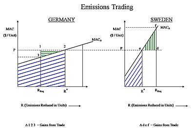
Example MACs for two different countries
For this example let us assume that Germany can abate its CO
2 at a much cheaper cost than Sweden, e.g. MAC
S > MAC
G where the MAC curve of Sweden is steeper (higher slope) than that of Germany, and R
Req is the total amount of emissions that need to be reduced by a country.
On the left side of the graph is the MAC curve for Germany. R
Req is the amount of required reductions for Germany, but at R
Req the MAC
G curve has not intersected the market allowance price of CO
2 (market allowance price = P = λ). Thus, given the market price of CO
2 allowances, Germany has potential to profit if it abates more emissions than required.
On the right side is the MAC curve for Sweden. R
Req is the amount of required reductions for Sweden, but the MAC
S curve already intersects the market price of CO
2 allowances before R
Req has been reached. Thus, given the market allowance price of CO
2, Sweden has potential to make a cost saving if it abates fewer emissions than required internally, and instead abates them elsewhere.
In this example, Sweden would abate emissions until its MAC
S intersects with P (at R*), but this would only reduce a fraction of Sweden’s total required abatement. After that it could buy emissions credits from Germany for the price
P (per unit). The internal cost of Sweden’s own abatement, combined with the credits it buys in the market from Germany, adds up to the total required reductions (R
Req) for Sweden. Thus Sweden can make a saving from buying credits in the market (Δ d-e-f). This represents the "Gains from Trade", the amount of additional expense that Sweden would otherwise have to spend if it abated all of its required emissions by itself without trading.
Germany made a profit on its additional emissions abatement, above what was required: it met the regulations by abating all of the emissions that was required of it (R
Req). Additionally, Germany sold its surplus to Sweden as credits, and was paid
P for every unit it abated, while spending less than
P. Its total revenue is the area of the graph (R
Req 1 2 R*), its total abatement cost is area (R
Req 3 2 R*), and so its net benefit from selling emission credits is the area (Δ 1-2-3) i.e. Gains from Trade
The two R* (on both graphs) represent the efficient allocations that arise from trading.
- Germany: sold (R* - RReq) emission credits to Sweden at a unit price P.
- Sweden bought emission credits from Germany at a unit price P.
If the total cost for reducing a particular amount of emissions in the
Command Control scenario is called
X, then to reduce the same amount of combined pollution in Sweden and Germany, the total abatement cost would be less in the
Emissions Trading scenario i.e. (X — Δ 123 - Δ def).
The example above applies not just at the national level: it applies just as well between two companies in different countries, or between two subsidiaries within the same company.
[edit] Applying the economic theory
The nature of the pollutant plays a very important role when policy-makers decide which framework should be used to control pollution.
CO
2 acts globally, thus its impact on the environment is generally similar wherever in the globe it is released. So the location of the originator of the emissions does not really matter from an environmental standpoint.
[34]
The policy framework should be different for regional pollutants
[35] (e.g.
SO2 and
NOX, and also mercury) because the impact exerted by these pollutants may not be the same in all locations. The same amount of a regional pollutant can exert a very high impact in some locations and a low impact in other locations, so it does actually matter where the pollutant is released. This is known as the
Hot Spot problem.
A
Lagrange framework is commonly used to determine the least cost of achieving an objective, in this case the total reduction in emissions required in a year. In some cases it is possible to use the Lagrange optimization framework to determine the required reductions for each country (based on their MAC) so that the total cost of reduction is minimized. In such a scenario, the
Lagrange multiplier represents the market allowance price (P) of a pollutant, such as the current market allowance price of emissions in Europe and the USA.
[36]
Countries face the market allowance price that exists in the market that day, so they are able to make individual decisions that would minimize their costs while at the same time achieving regulatory compliance. This is also another version of the
Equi-Marginal Principle, commonly used in economics to choose the most economically efficient decision.
[edit] Prices versus quantities, and the safety valve
There has been longstanding debate on the relative merits of
price versus
quantity instruments to achieve emission reductions.
[37]
An emission cap and permit trading system is a
quantity instrument because it fixes the overall emission level (quantity) and allows the price to vary. Uncertainty in future supply and demand conditions (market volatility) coupled with a fixed number of pollution credits creates an uncertainty in the future price of pollution credits, and the industry must accordingly bear the cost of adapting to these volatile market conditions. The burden of a volatile market thus lies with the industry rather than the controlling agency, which is generally more efficient. However, under volatile market conditions, the ability of the controlling agency to alter the caps will translate into an ability to pick "winners and losers" and thus presents an opportunity for corruption.
In contrast, an
emission tax is a
price instrument because it fixes the price while the emission level is allowed to vary according to economic activity. A major drawback of an emission tax is that the environmental outcome (e.g. a limit on the amount of emissions) is not guaranteed. On one hand, a tax will remove capital from the industry, suppressing possibly useful economic activity, but conversely, the polluter will not need to hedge as much against future uncertainty since the amount of tax will track with profits. The burden of a volatile market will be borne by the controlling (taxing) agency rather than the industry itself, which is generally less efficient. An advantage is that, given a uniform tax rate and a volatile market, the taxing entity will not be in a position to pick "winners and losers" and the opportunity for corruption will be less.
Assuming no corruption and assuming that the controlling agency and the industry are equally efficient at adapting to volatile market conditions, the best choice depends on the sensitivity of the costs of emission reduction, compared to the sensitivity of the benefits (i.e., climate damages avoided by a reduction) when the level of emission control is varied.
Because there is high uncertainty in the compliance costs of firms, some argue that the optimum choice is the price mechanism. However, the burden of uncertainty cannot be eliminated, and in this case it is shifted to the taxing agency itself.
Some scientists have warned of a threshold in atmospheric concentrations of carbon dioxide beyond which a run-away
warming effect could take place, with a large possibility of causing irreversible damages. If this is a conceivable risk then a quantity instrument could be a better choice because the quantity of emissions may be capped with a higher degree of certainty. However, this may not be true if this risk exists but cannot be attached to a known level of GHG concentration or a known emission pathway.
[38]
A third option, known as a
safety valve, is a hybrid of the price and quantity instruments. The system is essentially an emission cap and permit trading system but the maximum (or minimum) permit price is capped. Emitters have the choice of either obtaining permits in the marketplace or purchasing them from the government at a specified trigger price (which could be adjusted over time). The system is sometimes recommended as a way of overcoming the fundamental disadvantages of both systems by giving governments the flexibility to adjust the system as new information comes to light. It can be shown that by setting the trigger price high enough, or the number of permits low enough, the safety valve can be used to mimic either a pure quantity or pure price mechanism.
[39]
All three methods are being used as policy instruments to control greenhouse gas emissions: the EU-ETS is a
quantity system using the cap and trading system to meet targets set by
National Allocation Plans;
Denmark has a price system using a
carbon tax (World Bank, 2010, p. 218),
[40] while China uses the CO
2 market price for funding of its
Clean Development Mechanism projects, but imposes a
safety valve of a minimum price per tonne of CO
2.
[edit] Carbon leakage
Carbon leakage is the effect that regulation of emissions in one country/sector has on the emissions in other countries/sectors that are not subject to the same regulation (Barker
et al.., 2007).
[41] There is no consensus over the magnitude of long-term carbon leakage (Goldemberg
et al., 1996, p. 31).
[42]
In the Kyoto Protocol, Annex I countries are subject to caps on emissions, but non-Annex I countries are not. Barker
et al.. (2007) assessed the literature on leakage. The leakage rate is defined as the increase in CO
2 emissions outside of the countries taking domestic mitigation action, divided by the reduction in emissions of countries taking domestic mitigation action. Accordingly, a leakage rate greater than 100% would mean that domestic actions to reduce emissions had had the effect of increasing emissions in other countries to a greater extent, i.e., domestic mitigation action had actually led to an increase in global emissions.
Estimates of leakage rates for action under the Kyoto Protocol ranged from 5 to 20% as a result of a loss in price competitiveness, but these leakage rates were viewed as being very uncertain.
[43] For energy-intensive industries, the beneficial effects of Annex I actions through technological development were viewed as possibly being substantial. This beneficial effect, however, had not been reliably quantified. On the empirical evidence they assessed, Barker
et al.. (2007) concluded that the competitive losses of then-current mitigation actions, e.g., the EU ETS, were not significant.
One of the controversies about carbon mitigation policy thus arises about how to "level the playing field" with border adjustments.
[44] One component of the
American Clean Energy and Security Act, for example, along with several other energy bills put before Congress, calls for carbon surcharges on goods imported from countries without cap-and-trade programs. Even aside from issues of compliance with the
General Agreement on Tariffs and Trade, such border adjustments presume that the producing countries bear responsibility for the carbon emissions.
A general perception among developing countries is that discussion of climate change in trade negotiations could lead to "green
protectionism" by high-income countries (World Bank, 2010, p. 251).
[40] Tariffs on imports ("virtual carbon") consistent with a carbon price of $50 per ton of CO
2 could be significant for developing countries. World Bank (2010) commented that introducing border tariffs could lead to a proliferation of trade measures where the competitive playing field is viewed as being uneven. Tariffs could also be a burden on low-income countries that have contributed very little to the problem of climate change.


